The infinite relational model (IRM) explains a graph by grouping its nodes, and it decides how many groups to use. This post builds the collapsed Gibbs sampler for it one step at a time, and ends with code you can run.
The generative story
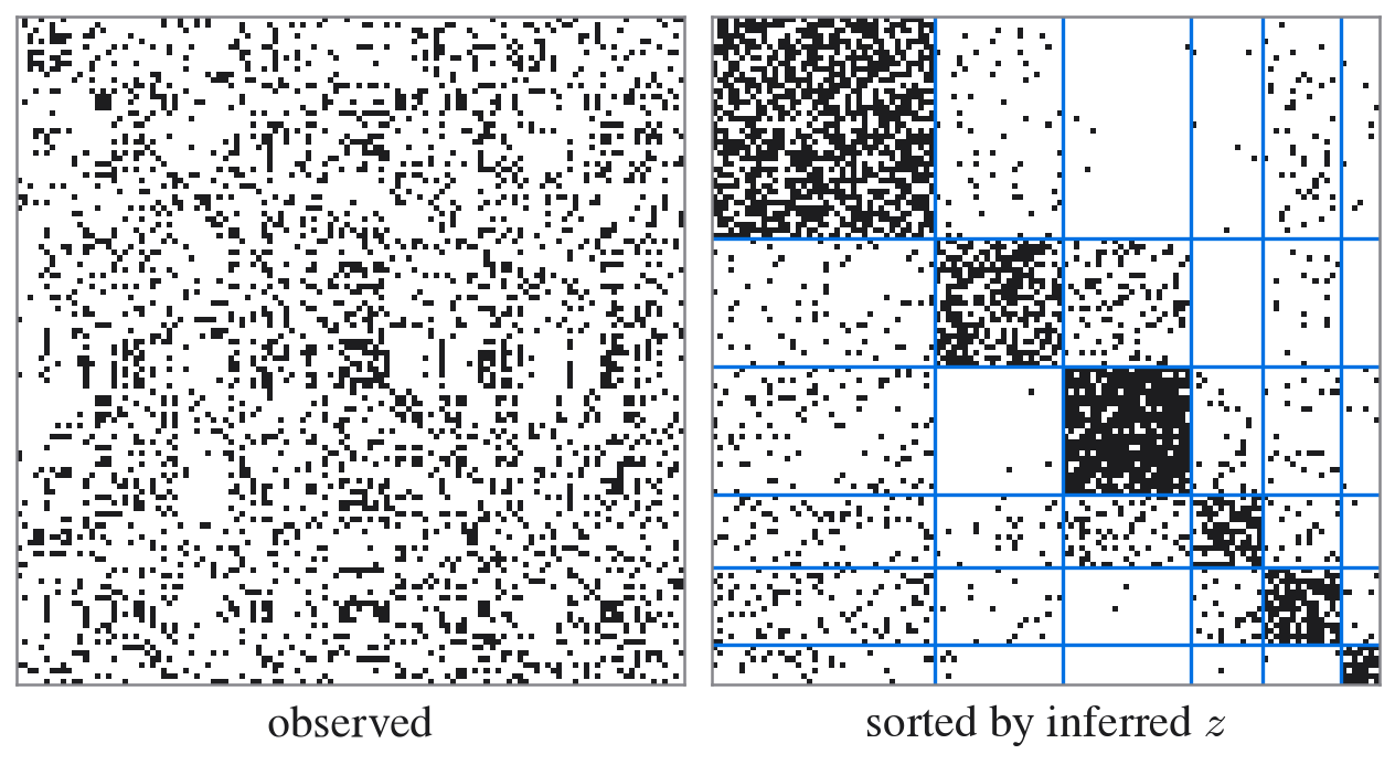
Every node $i$ gets a cluster label $z_i$ from a Chinese restaurant process. Each pair of clusters $(k,l)$ gets a link probability $\theta_{kl}$, and each edge is a coin flip with the probability of its two clusters:
$$z \sim \mathrm{CRP}(\alpha), \qquad \theta_{kl} \sim \mathrm{Beta}(a, b), \qquad x_{ij} \mid z, \theta \sim \mathrm{Bernoulli}\big(\theta_{z_i z_j}\big).$$Two lookups connect the matrices: node $i$ has label $k = z_i$, node $j$ has label $l = z_j$, and the edge $x_{ij}$ uses entry $\theta_{kl}$. The number of clusters $K$ is not a parameter. It is simply the number of distinct labels in $z$.
Integrate out $\theta$
Because the Beta prior is conjugate to the Bernoulli likelihood, $\theta$ can be integrated out. What remains depends on two counts per cluster pair: $n_{kl}$, the number of links, and $\bar n_{kl}$, the number of non-links. The marginal likelihood of a block is a ratio of Beta functions, $B(a + n_{kl},\, b + \bar n_{kl}) / B(a, b)$.
One Gibbs step
Take node $i$ out of its cluster and update the counts. Let $m_k^{-i}$ be the size of cluster $k$ without $i$, and let $n^{(i)}_{kl}$ and $\bar n^{(i)}_{kl}$ be the links and non-links that $i$ would add to block $(k,l)$. Then
$$p(z_i = k \mid z_{-i}, X) \;\propto\; m_k^{-i} \prod_{l} \frac{B\big(a + n_{kl}^{-i} + n^{(i)}_{kl},\; b + \bar n_{kl}^{-i} + \bar n^{(i)}_{kl}\big)}{B\big(a + n_{kl}^{-i},\; b + \bar n_{kl}^{-i}\big)},$$and a brand-new cluster gets weight $\alpha \prod_l B(a + n^{(i)}_{l},\, b + \bar n^{(i)}_{l}) / B(a,b)$. Sample $z_i$ from these weights, put $i$ back, and move to the next node. One pass over all nodes is a sweep. In practice every term is computed in log space with gammaln, so the products become sums.
Run it
from isbm import generate_irm_graph, CGS_IRM
from isbm.metrics import ari

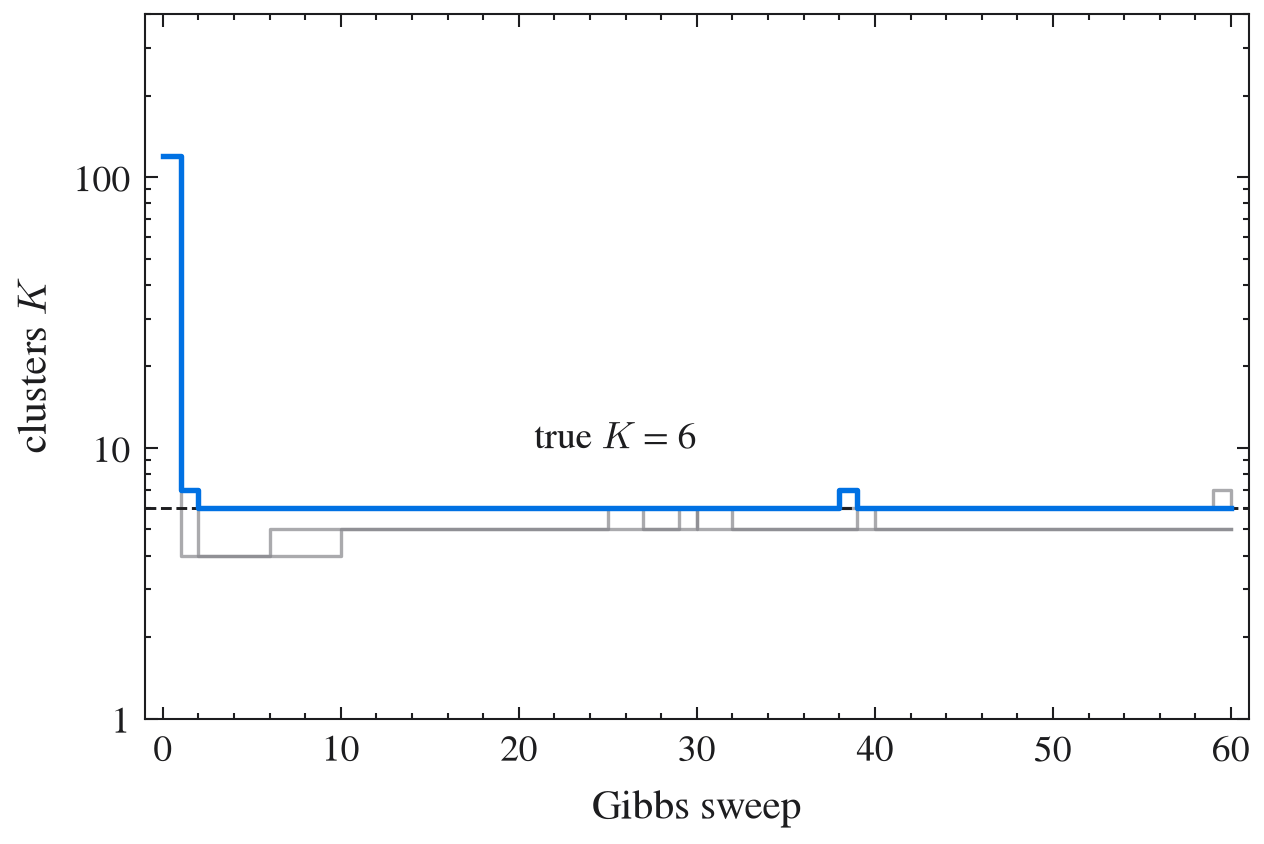
X, z = generate_irm_graph(N=120, alpha=1.5, seed=170)
model = CGS_IRM(n_iter=60, burnin=0, seed=0).fit(X)
print(ari(z, model.z1_))   # 1.0 on this graph
[Look back: what surprised you, what breaks the sampler (e.g. bad hyperparameters, slow mixing), and what you'd try next.]
References
- C. Kemp et al. Learning systems of concepts with an infinite relational model. AAAI, 2006.
- K. Ishiguro, I. Sato and N. Ueda. Averaged collapsed variational Bayes inference. JMLR 18, 2017 (arXiv:1409.4757).